|
Getting your Trinity Audio player ready…
|
To address your request, I’ll interpret it as asking for a graph that generalizes the relationship between the perceived probability of an event (e.g., the probability one might assume based on a test result or evidence, often naively taken as the test’s accuracy) and the actual probability of the event being true, given new evidence, across varying prior probabilities. This generalizes the previous disease-testing scenario to any event where Bayesian reasoning applies, such as medical tests, spam filters, or quality control checks.
Conceptual Framework
- Perceived Probability: This is often the test’s reported accuracy (e.g., sensitivity, or the probability of a positive result given the event is true). For simplicity, let’s assume people perceive the probability of the event being true as equal to the test’s sensitivity (e.g., 99% for a positive test result), ignoring the prior probability or false positives.
- Actual Probability: This is the posterior probability, calculated using Bayes’ theorem, which depends on the prior probability of the event and the test’s accuracy (sensitivity and specificity).
- Generalized Setup: We’ll use the same test parameters as before (99% sensitivity and specificity) to maintain continuity, but frame it as any event (not just a disease). The x-axis will represent the prior probability of the event (from 0 to 1), and the y-axis will compare the perceived probability (fixed at 99% for a positive result) versus the actual posterior probability (computed via Bayes’ theorem).
Assumptions
- Test parameters:
- Sensitivity (( P(Pos|E) )) = 0.99 (probability of a positive result given the event is true).
- Specificity = 0.99, so False Positive Rate (( P(Pos|not E) )) = 0.01.
- Perceived probability: Assume people naively interpret a positive result as meaning there’s a 99% chance the event is true (i.e., equating it to the test’s sensitivity, ( P(Pos|E) = 0.99 )).
- Actual probability: The posterior probability, ( P(E|Pos) ), calculated as:
[
P(E|Pos) = \frac{P(Pos|E) \cdot P(E)}{P(Pos|E) \cdot P(E) + P(Pos|not E) \cdot P(not E)}
]
where ( P(E) ) is the prior probability of the event, and ( P(not E) = 1 – P(E) ). - Graph: The x-axis will be the prior probability (( P(E) )), and the y-axis will show two lines:
- Perceived probability: A flat line at 99% (0.99), representing the naive assumption.
- Actual probability: The posterior probability ( P(E|Pos) ), which varies with the prior.
Data Points
Using the same calculations as in the previous response for consistency:
- For ( P(E) = 0.001 ): ( P(E|Pos) \approx 0.0902 ) (9.02%).
- For ( P(E) = 0.01 ): ( P(E|Pos) = 0.5 ) (50%).
- For ( P(E) = 0.1 ): ( P(E|Pos) \approx 0.9167 ) (91.67%).
- For ( P(E) = 0.2 ): ( P(E|Pos) \approx 0.9615 ) (96.15%).
- For ( P(E) = 0.3 ): ( P(E|Pos) \approx 0.9756 ) (97.56%).
- For ( P(E) = 0.4 ): ( P(E|Pos) \approx 0.9836 ) (98.36%).
- For ( P(E) = 0.5 ): ( P(E|Pos) = 0.99 ) (99%).
- For ( P(E) = 0.6 ): ( P(E|Pos) \approx 0.9945 ) (99.45%).
- For ( P(E) = 0.7 ): ( P(E|Pos) \approx 0.9972 ) (99.72%).
- For ( P(E) = 0.8 ): ( P(E|Pos) \approx 0.9987 ) (99.87%).
- For ( P(E) = 0.9 ): ( P(E|Pos) \approx 0.9989 ) (99.89%).
- Perceived probability: Constant at 0.99 (99%) for all ( P(E) ).
Chart Creation
I’ll create a line chart with two datasets:
- Perceived Probability: A horizontal line at 99%.
- Actual Probability: The posterior probability ( P(E|Pos) ), varying with the prior ( P(E) ).
{
  "type": "line",
  "data": {
    "labels": [0.1, 1, 10, 20, 30, 40, 50, 60, 70, 80, 90],
    "datasets": [
      {
        "label": "Perceived Probability (%)",
        "data": [99, 99, 99, 99, 99, 99, 99, 99, 99, 99, 99],
        "borderColor": "#FF5733",
        "backgroundColor": "rgba(255, 87, 51, 0.2)",
        "fill": false,
        "tension": 0
      },
      {
        "label": "Actual Probability (%)",
        "data": [9.02, 50, 91.67, 96.15, 97.56, 98.36, 99, 99.45, 99.72, 99.87, 99.89],
        "borderColor": "#4CAF50",
        "backgroundColor": "rgba(76, 175, 80, 0.2)",
        "fill": false,
        "tension": 0.4
      }
    ]
  },
  "options": {
    "scales": {
      "x": {
        "title": {
          "display": true,
          "text": "Prior Probability of Event (%)"
        },
        "min": 0,
        "max": 100
      },
      "y": {
        "title": {
          "display": true,
          "text": "Probability (%)"
        },
        "min": 0,
        "max": 100
      }
    },
    "plugins": {
      "legend": {
        "display": true
      }
    }
  }
}
Explanation of the Chart
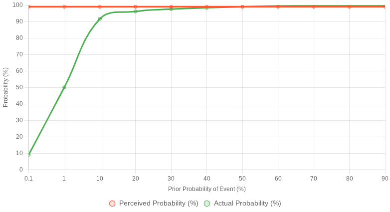
- X-axis: The prior probability of the event (( P(E) )), expressed as a percentage (0% to 100%). This represents how common the event is before considering the test result (e.g., disease prevalence, probability of an email being spam, etc.).
- Y-axis: The probability (in percentage) of the event being true, comparing:
- Perceived Probability: A flat line at 99%, reflecting the naive assumption that a positive test result means a 99% chance the event is true (based on the test’s 99% sensitivity).
- Actual Probability: The posterior probability ( P(E|Pos) ), which starts low (e.g., 9.02% when the prior is 0.1%) and rises toward 99% as the prior increases.
- Key Insight: When the event is rare (low prior, e.g., 0.1%), the actual probability is much lower than the perceived 99% due to false positives. As the prior probability increases, the actual probability approaches the perceived probability, converging at 99% when the prior is 50% or higher.
- Generalized Interpretation: This chart applies to any scenario where a test or evidence (with 99% sensitivity and specificity) is used to assess an event’s likelihood. For rare events (low prior), the actual probability is far lower than what one might assume from the test’s accuracy alone, emphasizing the importance of Bayesian reasoning in interpreting evidence.
This graph highlights the disconnect between naive perceptions (overestimating probability based on test accuracy) and the actual probability, which depends heavily on the prior probability of the event.
Leave a Reply