|
Getting your Trinity Audio player ready…
|
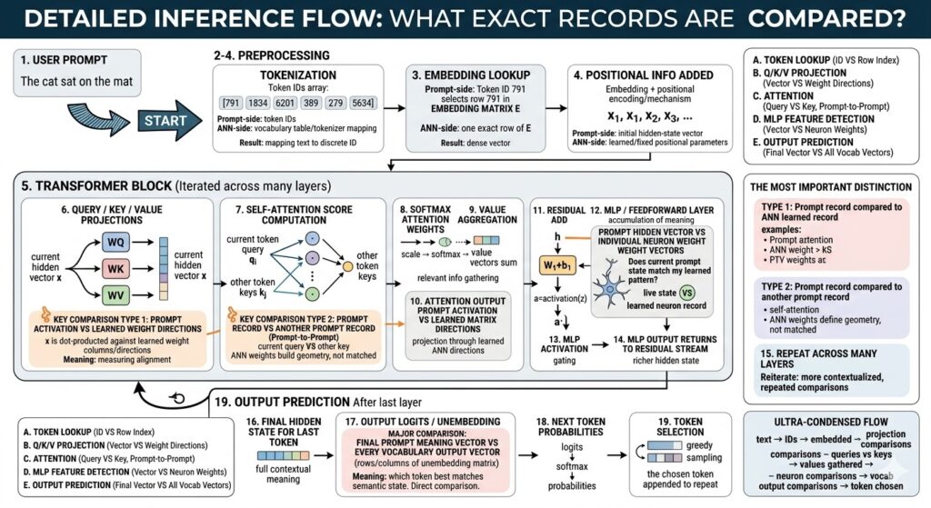
Here are explanations for each labeled processing block:
Block 1: USER PROMPT
This block marks the input stage of the inference process. The entire pipeline begins when natural language text, such as “The cat sat on the mat,” is provided. This raw data cannot be understood directly by a neural network. At this point, no similarity comparison occurs. The system is simply receiving the textual request as raw input, which it will then pass to the pre-processing stages to be converted into a machine-readable format for subsequent vector analysis and comparison against learned model parameters.
Block 2: TOKENIZATION
This is the first pre-processing block. The raw user prompt is segmented into smaller units called tokens (words, sub-words, or characters). Each unique token maps to a specific, unique numerical Token ID. The comparison here is not mathematical similarity, but a definitive lookup of the prompt text against a learned ANN-side vocabulary table and tokenizer mapping. The result is a discrete array of numbers, transforming the text into structured data like [791, 1834, 6201, 389, 279, 5634], preparing it for subsequent high-dimensional vector transformation.
Block 3: EMBEDDING LOOKUP
After tokenization, each Token ID is converted into a high-dimensional, dense semantic vector. This conversion is the embedding lookup. Each discrete ‘prompt-side record’ (Token ID) serves as an exact index into a pre-trained ANN-side database: the learned embedding matrix E. This is not a fuzzy match or similarity search (like dot-product similarity); it is a precise direct selection process. The prompt token ID selects a specific, exact row from the stored ANN records, resulting in a continuous vector that represents the core semantic meaning of that single token.
Block 4: POSITIONAL INFORMATION ADDED
Since raw semantic embeddings don’t carry sequence order, positional information must be added. This visual block shows that a vector representing token position (from learned or fixed parameters) is combined with (often added to) the semantic embedding. The resulting prompt-side record is the initial hidden-state vector for each token position (x₁, x₂, x₃…), now representing both semantic meaning and exact sequence location. This stage is primarily a transformation through vector addition, not a competitive match search or similarity comparison between records.
Block 5: TRANSFORMER BLOCK (Iterated across many layers)
This visual block wraps the main computational engine iterated over many layers. At every layer, hidden vectors enter repeated comparisons to become more contextualized. These recurrent comparisons are: (1) live prompt hidden vectors against learned weight columns (identifying expression of features); (2) a token’s Query vector against other tokens’ Key vectors (determining relevance to context); and (3) hidden vectors against MLP neuron weight vectors (pattern matching). This iteration refines the token representations, asking deeper questions about semantic alignment and contextual relevance across dozens of stacked processing stages.
Block 6: QUERY / KEY / VALUE PROJECTIONS
This block highlights one of the first true record-to-record comparisons of inference. The live prompt-side hidden vector x is dot-producted against the learned columns and directions inside WQ, WK, and WV weight matrices (ANN-side learned records). Each matrix creates separate Query, Key, and Value vectors. This calculation involves multiplying the live prompt activation against learned ANN weight directions. Every output component effectively measures the strength of alignment, asking: “How much does the current prompt state express this specific learned feature direction?”
Block 7: SELF-ATTENTION SCORE COMPUTATION
Here, the model performs a definitive prompt-to-prompt comparison. For the current token i, its Query vector (qi) is compared against the Key vectors (kj) of all other allowed positions within the prompt sequence (a prompt-derived record compared to other prompt-derived records). The comparison is another dot product: score(i,j) = qi · kj. Crucially, learned ANN weights were used only to create the geometric coordinate system for this comparison, and are not matched here. The model effectively asks: “Which other parts of the current context are most important right now?”
Block 8: SOFTMAX ATTENTION WEIGHTS
This block visualizes the conversion of raw scores into relevance percentages. No new record-to-record comparison occurs at this stage. Following self-attention score computation, the raw scores for all key-query comparisons are scaled, and then passed through a mathematical softmax function. This normalizes the scores so that all results are between 0 and 1, and sum to 1.0. This non-comparative functional step converts raw similarity values into structured probabilities (attention weights), directly defining exactly how much focus should be assigned to every other allowed token position.
Block 9: VALUE AGGREGATION
In this block, contextual information is gathered into a single representation. The prompt-side attention weights (from step 8) and prompt-side Value vectors (vj, derived in step 6 from other positions) are mathematically combined through a weighted sum: attention_output(i) = Σ softmax(qi·kj) · vj. While ANN records (specifically WV) created the geometry for the initial value vectors, this calculation is an aggregation of prompt-derived information. The meaning of this process is that context is mathematically gathered into a refined representation, guided by the token-to-token relevance found in step 7.
Block 10: ATTENTION OUTPUT PROJECTION
Following self-attention, the aggregated attention output vector for each token must be projected through another learned ANN matrix. This prompt-derived record is dot-producted with the learned directions of the output projection matrix WO. This step involve multiplying the live, prompt activation against learned ANN weight directions, not a competitive matching search. Instead, the model is projecting the aggregated information, shaping it against stored model records as it prepares to enter the next major processing layer, adding another layer of contextual alignment refinement.
Block 11: RESIDUAL ADD
Modern Transformers include “residual connections” to accumulate meaning across layers. In this non-comparative mathematical addition, the original hidden state vector for a token (which was input to self-attention) is added to the newly refined attention update vector from step 10. This step involves no similarity comparison; it is an accumulation of meaningful information rather than a “match search.” The result ensures that core information from previous processing stages is preserved and contextualized, rather than overwritten, during the repeated alignment calculations.
Block 12: MLP / FEEDFORWARD LAYER
This block contains a crucial comparison of live data against neuron patterns. The hidden vector h enters a multi-layer perceptron (MLP). In the first MLP stage, z = h · W1 + b1, the prompt hidden vector (h) is compared via dot product with individual neuron weight vectors. This is a definitive example of live prompt state vs learned ANN neuron record. Each neuron effectively asks: “How much does the current prompt state match my specific learned pattern?” Strong alignment causes the neuron to activate strongly, determining which semantic features influence next-token prediction.
Block 13: MLP ACTIVATION
This functional block gates which matched learned semantic features are important. After the MLP dot product comparison, a non-linear activation function is mathematically applied. No new comparison beyond the computed dot products occurs at this stage. Instead, this non-linearity processes the scores, causing some feature detectors (neurons) to express a strong activation, indicating a strong match to their learned patterns, while others remain weak or near zero. In effect, it filters the results of previous record-vs-record pattern matching.
Block 14: MLP OUTPUT RETURNS TO RESIDUAL STREAM
Similar to Block 11, this step acts as a final non-comparative mathematical accumulation of refined meaning. The final resulting output vector from the entire MLP layer is added to the current hidden state which was preserved earlier. The process involves no competitive match or similarity search; it is an aggregation of computed information. This addition ensures that the token’s representation now carries both its prior history and the rich, contextualized information derived from the most recent comparison loops.
Block 15: REPEAT ACROSS MANY LAYERS
The core power of Transformers is derived from repeated iteration. The visual arrow highlights that the main processing blocks (6–14) are not a single event but are iterated over stacked layers. At every layer, the prompt-side records (the hidden vectors) become more complex and contextualized. Repeated comparisons include: hidden vector vs learned projection weight directions; token query vs key (prompt-to-prompt); and hidden vector vs learned MLP neuron weight patterns. Each stacked layer refines these comparisons, progressively building complex semantic representations and identifying deeper connections in the context.
Block 16: FINAL HIDDEN STATE FOR LAST TOKEN
After the sequence passes through all stacked iterations, the system is ready for prediction. This visual block represents the complex, final context-rich prompt-side vector for the sequence’s last position. This vector is no longer a simple embedding of the original text; it is a highly contextualized semantic representation, embodying the final semantic state of the entire prompt and previous output sequence. This unique, complex record is the culmination of all previous comparisons, serving as the live data that will now be competitive matched for word prediction.
Block 17: OUTPUT LOGITS / UNEMBEDDING
In this block, the model’s final refined semantic state is compared to every possible word in the vocabulary. The calculation is final_hidden · W_vocab^T. The single, complex, final prompt-meaning vector is compared via dot product against every individual output vector in the learned ANN-side vocabulary unembedding matrix. This is another highly definitive direct competitive comparison. It effectively asks: “Which vocabulary token direction best matches the semantic state described by this final vector?” determining the relative raw probability score (logit) for every potential next word.
Block 18: NEXT TOKEN PROBABILITIES
This block functionalizes raw scores into probabilities. No new record-vs-record comparison occurs. The raw logits (from step 17) are processed by scaling and then passed through a mathematical softmax function. This normalizes all candidate scores so they all lie strictly between 0 and 1, and sum precisely to 1.0. This step provides the statistical probability distribution for the next token, converting the fuzzy similarity scores into the structured percentages required for the selection logic, highlighting the probabilistic approach of text generation.
Block 19: TOKEN SELECTION
This is the final decision and loop point. Once probabilities are assigned, a specific token is selected based on a decoding strategy (greedy decoding, sampling, beam logic, etc.). The chosen token is visually appended to the existing sequence. For text generation to continue, this appended token becomes part of the sequence and the entire cycle begins again, treating the extended sequence as the new prompt. This specific decision stage involves no comparative match of records; it is purely a decision, action, and loop point.
THE MOST IMPORTANT DISTINCTION
This summary block defines the two core comparison categories essential for understanding the model:
Type 1 involves comparing a live “prompt activation” against pre-trained “learned weight directions” through multiplication. Examples include hidden vectors vs MLP neuron weights or final vectors vs vocabulary vectors, effectively measuring semantic alignment.
Type 2 involves comparing one “prompt record” to another “prompt record” through self-attention (current query vs earlier keys). In this process, ANN weights define the learned geometry but are not directly matched, highlighting prompt-to-prompt relevance.
Leave a Reply