|
Getting your Trinity Audio player ready…
|
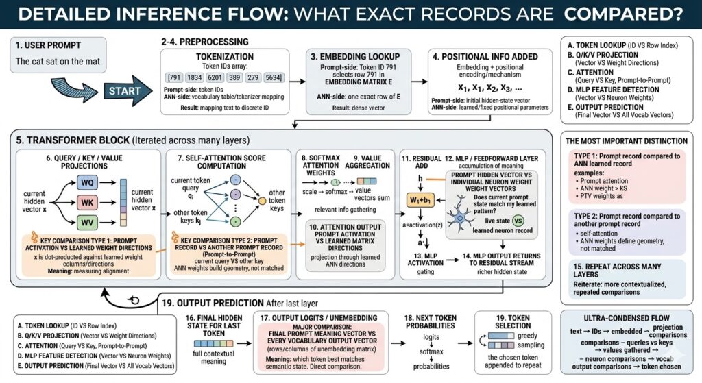
Block 1: USER PROMPT
This is the human-facing beginning of the entire inference event. A user types something in ordinary language, such as “The cat sat on the mat,” and to the human mind that already feels like meaning. But to the model, at this instant, it is not yet meaning in any computational sense. It is simply raw symbolic input arriving from outside the network. The crucial point is that the model does not “read” text the way a person does. It cannot directly ingest letters or words as meaningful objects. It must first transform the prompt into internal representations the network can operate on. Your original description emphasizes that no true similarity comparison happens yet, and that is exactly right: this stage is reception, not interpretation. (LF Yadda – A Blog About Life)
At this point, the prompt is still in the format of visible characters. It lives in the domain of typography and language encoding, not yet in the domain of vectors and learned feature geometry. The system has not asked whether one phrase resembles another. It has not compared the prompt to memories. It has not searched for semantic neighbors. It has not activated neurons in any deep sense. Instead, the system is standing at the doorway of the model pipeline, holding a raw string that must be converted into a structured machine-processable form.
This matters because people often imagine that an LLM instantly “understands” the question. But understanding in an LLM is not a magical first event. It is an emergent consequence of multiple later transformations. The user prompt block therefore marks the boundary between the outside symbolic world and the inside computational world. It is where language enters the machine, but not yet where language becomes machine meaning.
Another important distinction is that the prompt arrives as a sequence. Even before the model analyzes meaning, the ordering of characters and words is already there in the human text. That order will eventually matter immensely, but the model cannot use it until later stages convert the text into token identities and position-aware vectors. So this first block is like handing a document to a translator who has not opened it yet. The information is present, but its operational form has not been unlocked.
In practical systems, this stage may include text normalization steps outside the core neural network, such as handling Unicode, special characters, or system instructions. But conceptually the essence remains simple: the user supplies language, and the model pipeline receives it as input material. It is raw fuel, not yet combustion. It is the spoken question before it becomes mathematics. It is the semantic seed before it enters the geometry of inference. Your post frames this correctly as the true beginning of the pipeline but not yet the beginning of comparison, and that distinction is foundational for understanding everything that follows. (LF Yadda – A Blog About Life)
Block 2: TOKENIZATION
Tokenization is the first real act of machine-side structuring. The system takes the raw prompt string and breaks it into smaller units called tokens. These are not always full words. Depending on the tokenizer, a token may be a complete word, a word fragment, punctuation mark, number chunk, or even a rare-character segment. Your original explanation makes the key point that the action here is not fuzzy similarity search but exact lookup against a vocabulary and tokenizer mapping. That is exactly the right way to frame it. Tokenization is categorical, not semantic. The system is not yet asking what the text means; it is asking how to segment it into recognized symbolic pieces. (LF Yadda – A Blog About Life)
Each token is then mapped to a unique token ID. This is a discrete identifier, not a vector. If the prompt contains six token units, the result is a sequence of six integers. Those integers are machine handles that refer to entries in the model’s vocabulary. The important idea is that this process is deterministic once the tokenizer and vocabulary are fixed. The token “cat” does not search for the most similar vocabulary item. It maps to the vocabulary entry the tokenizer defines for that text pattern. This is closer to indexing a dictionary than to measuring semantic closeness.
Why does this matter? Because it explains a central divide inside LLM inference. Early in the pipeline, language is handled as symbolic categories. Later in the pipeline, those categories become continuous vectors in high-dimensional space. Tokenization is the bridge between raw text and numeric identifiers, but it is still on the symbolic side of that divide. The model has not yet entered its true semantic geometry.
Tokenization also explains many strange behaviors users observe. A long word may split into several tokens. A rare name may break into unusual fragments. Two phrases that look similar to a person may tokenize differently, creating different downstream trajectories in the model. This is one reason prompting can be sensitive to wording. The tokenizer defines the discrete pieces that the rest of the model must work with.
Another subtle point is that tokenization compresses the infinite variety of possible input strings into a finite working vocabulary plus composition rules. The network cannot have a separate primitive symbol for every possible sentence. Instead, it builds sentences from token pieces. In effect, tokenization provides the alphabet of the model’s internal language. That alphabet is numeric, not semantic, but it is the necessary precondition for later semantic processing.
So tokenization is best understood as the mechanical segmentation and naming phase. It cuts the flowing stream of human text into addressable units. It assigns each unit a stable symbolic code. It prepares the prompt for embedding lookup by converting language into discrete machine-recognizable identities. That is why your original post is right to stress that the comparison here is a definite lookup, not a similarity judgment. The machine is not yet deciding what the prompt is like. It is deciding what the prompt is made of. (LF Yadda – A Blog About Life)
Block 3: EMBEDDING LOOKUP
Embedding lookup is the moment the prompt crosses from discrete symbol IDs into continuous vector space. After tokenization, each token is represented only as an integer ID. That number by itself carries no rich semantic structure. It is simply an address. The embedding matrix is what turns that address into a learned high-dimensional vector. Your post correctly emphasizes that this is still not a fuzzy search. The token ID indexes an exact row of the learned embedding table. The operation is precise selection, not approximate matching. (LF Yadda – A Blog About Life)
This distinction is extremely important because many people imagine embeddings are created on the fly by “thinking” about the token. In standard transformer inference, the embedding for a token is already stored in the model parameters. When the token ID arrives, the model retrieves the corresponding row from the embedding matrix. That row is a dense vector, often with hundreds or thousands of dimensions. Each dimension is not directly human-readable, but together the dimensions place the token at a learned location in semantic space.
The power of this step is that it transforms a hard category into a soft geometry. A token ID like 1834 is a rigid symbolic label. Its embedding vector is a pattern of continuous values that can participate in linear algebra. Once the token is represented as a vector, it can be added to other vectors, projected through matrices, compared by dot products, and shaped by downstream transformations. This is when the model leaves the world of dictionary indexing and enters the world of distributed meaning.
It is tempting to think of the embedding vector as “the meaning” of the token, but that is only partly true. A better way to say it is that the vector is the model’s learned starting representation for that token. It encodes statistical and relational tendencies derived from training. Tokens used in similar contexts tend to end up in related regions of embedding space. So the embedding is not a definition in the dictionary sense. It is more like a compressed coordinate in a learned semantic field.
Another subtle point is that embedding lookup happens independently for each token. At this stage, the token “cat” gets the same base embedding whether it appears in “the cat slept” or “the cat engine failed,” assuming it tokenizes the same way. Context has not yet altered it. That will happen later in the transformer layers. So the embedding is a context-poor starting state, not the fully contextual meaning the model will eventually use.
This is why the embedding lookup block is such a profound transition. It is the first place where a prompt-side record becomes a vector-shaped resident of the model’s latent geometry. The token ID acts as the retrieval key, and the embedding matrix acts as the stored semantic seed bank. The result is not final understanding, but it is the first real mathematical form in which understanding can begin. Your post captures that cleanly: exact token IDs select exact learned rows, and those rows become the continuous semantic starting points for all later inference. (LF Yadda – A Blog About Life)
Block 4: POSITIONAL INFORMATION ADDED
A pure embedding vector tells the model something about token identity, but nothing about sequence order. If the model only received embeddings, then “dog bites man” and “man bites dog” would contain the same token identities with no built-in sense of arrangement. That is why positional information must be added. Your post describes this as combining a position vector with the semantic embedding, usually by vector addition, to create an initial hidden state that contains both meaning and location. That is precisely the right intuition. (LF Yadda – A Blog About Life)
This step is easy to overlook because it seems almost too simple. A position-derived vector is added to the token embedding, and suddenly the model has a way to distinguish first position from third, earlier token from later token. But conceptually, this is a major event. It means the model’s representation is no longer just “what token is this?” It becomes “what token is this, here?” The token’s identity and its place in the sequence are fused into one starting state.
Why addition? Because vector addition is a compact way of superimposing two kinds of information into a shared representational space. One vector says something about token identity. The other says something about location. The sum becomes the token’s initial coordinate in the residual stream. Later layers can learn to extract and use both components. This is not a competition between records, as your post notes. It is a constructive synthesis.
Positional information can be implemented in different ways. Some models use fixed sinusoidal patterns. Others use learned positional embeddings. Still others use relative or rotary positional methods. But the common goal is the same: encode the structure of order so the transformer can reason over sequences rather than unordered bags of tokens. Without this, attention would know what tokens are present but not who comes before whom, who is adjacent to whom, or which token is the current position of interest.
This matters because language is inherently order-sensitive. Grammar, reference, cause and effect, quotation boundaries, and narrative flow all depend on sequence structure. Positional encoding gives the model a scaffold for this structure before any attention comparisons happen. It is the reason later self-attention can distinguish “look backward” from “look everywhere” and can meaningfully assign relevance to earlier versus later positions.
Another useful way to think about this block is that it creates the model’s initial hidden state stream. Before this step, there are token embeddings and separate positional signals. After this step, there is a unified sequence of vectors, one per token position, each carrying both lexical identity and structural placement. These vectors are the real working substrate of the transformer. From here onward, the network does not operate on raw words or IDs. It operates on these hidden states and their descendants.
So positional addition is not just a technical footnote. It is the act that converts isolated token meanings into sequence-aware starting states. It gives the model an internal sense of arrangement. It lets the system know not just what symbols arrived, but how they are laid out in time and order. That is why your original explanation is so important: no new similarity search occurs here. Instead, this block equips the model with the geometry of sequence itself, making all later contextual comparison possible. (LF Yadda – A Blog About Life)
Block 5: TRANSFORMER BLOCK (Iterated Across Many Layers)
This block is the heart of the model. Your post describes it as the main computational engine repeated over many layers, and that is exactly what a transformer is: not one magical reasoning step, but a stack of repeated refinement modules. Once the sequence of initial hidden states has been formed, these vectors enter a cycle of transformations that repeatedly compare, project, aggregate, and update them. The power does not come from any single pass. It comes from the accumulation of many passes, each deepening contextualization. (LF Yadda – A Blog About Life)
Inside each transformer block, several different kinds of comparison happen. First, live hidden states are projected against learned weight directions. This lets the model measure how strongly the current prompt state expresses certain learned features. Second, prompt-derived query vectors are compared with prompt-derived key vectors, allowing tokens to determine which other tokens matter most right now. Third, hidden states are tested against learned multilayer perceptron neuron patterns, enabling feature detection and nonlinear expansion. Your post rightly separates these comparison types instead of lumping everything together under the vague word “attention.”
This repeated structure is what allows contextual meaning to emerge. Early layers may focus on relatively local or literal relationships: nearby syntax, token identity disambiguation, phrase boundaries. Middle layers often build broader contextual patterns, such as semantic roles, discourse structure, or long-range dependencies. Later layers may compress the entire preceding sequence into a form optimized for prediction at the next token. While that layer-by-layer story varies by model and is never perfectly clean, the general principle holds: stacked transformer blocks progressively refine representation.
An important insight is that the hidden vector entering one block is not thrown away when the block updates it. Residual pathways let the model keep the prior state while adding new context-sensitive adjustments. This means each layer acts less like a replacement and more like an incremental interpretation pass. The representation becomes richer without losing the history of what it already was.
Another way to understand this block is to see it as a semantic metabolism engine. Each layer takes in current token representations, subjects them to interaction with both learned circuitry and current context, and emits updated representations that are more informed by the full sequence. The transformer block is where static learned structure meets dynamic prompt-specific activity. The weights are frozen knowledge about how to process patterns; the activations are the living state produced by this particular prompt.
Because the same basic machinery is repeated many times, the model can build depth. A single attention-and-MLP layer might notice only simple patterns. But dozens of such layers can construct hierarchies of abstraction, allowing the final hidden state to reflect not just word identity but relationships, implications, tone, context, and anticipated continuation.
So this block is not one operation but a chamber in a larger pipeline of repeated semantic refinement. Your original explanation captures the essence: the transformer block is where prompt records repeatedly interact with learned ANN-side structures and with one another, layer after layer, until a highly contextualized internal representation emerges. The model’s intelligence is not located in a single place inside this block. It is distributed across the iterative dance this block performs again and again. (LF Yadda – A Blog About Life)
Block 6: QUERY / KEY / VALUE PROJECTIONS
This is one of the first places where the model takes a current hidden state and actively reshapes it into multiple specialized forms for contextual comparison. Your post explains that the live hidden vector is multiplied by learned matrices WQ, WK, and WV to produce Query, Key, and Value vectors, and that each output component reflects alignment with learned feature directions. That is exactly the right interpretation. The model is not yet comparing token to token here; it is first constructing the coordinate systems and descriptors that will make token-to-token comparison possible. (LF Yadda – A Blog About Life)
The same hidden state enters three different learned linear maps. Why three? Because the model needs three distinct roles in attention. The Query vector represents what the current position is seeking or asking for. The Key vector represents what each position offers as an addressable relevance signature. The Value vector represents the content that will actually be passed along if that position is attended to. In other words: query asks, key identifies, value carries substance.
These projections are learned, which means the model has discovered during training how to transform a token’s current hidden state into useful attention-space representations. The original hidden state contains mixed information. The Q, K, and V projections disentangle that mixed information into different functional views. A token may carry many aspects at once: syntax, semantics, topic, role in sentence, referential importance. The projection matrices learn how to extract the aspects most useful for relevance scoring and information transfer.
It is important to stress that this stage is prompt-to-weight interaction, not prompt-to-prompt interaction. Each hidden state is being projected through stored matrices. So this is a comparison between live activation and learned ANN-side parameter structure. The dot products implicit in the matrix multiplication ask, feature by feature, how much the current hidden state aligns with each learned projection direction. The output is not yet an attention decision. It is the preparation of attention ingredients.
This block also reveals something deep about transformers: attention is not performed directly on raw embeddings or even raw hidden states. It is performed on transformed views of those hidden states. That means the model can learn different representational spaces for different heads and different layers. One attention head might learn to project hidden states in a way that highlights syntactic dependency. Another might highlight topic continuity. Another might focus on positional or referential cues. The learned projection matrices define those different lenses.
So the Q/K/V projection stage is like shaping raw contextual states into searchable profiles and retrievable payloads. It is where the model turns general-purpose hidden vectors into task-specific attention participants. Your original explanation is right to say that the output components measure expression along learned directions. That is the essence of linear projection in a trained model. The live prompt state is being asked: which aspects of your learned feature geometry are active right now, and how should those aspects be split into asking, identifying, and carrying roles? That is what makes the next stage of true token-to-token comparison possible. (LF Yadda – A Blog About Life)
Block 7: SELF-ATTENTION SCORE COMPUTATION
This is the signature operation of transformer architecture: one prompt-derived record is compared against other prompt-derived records. Your post states it very well: the current token’s Query vector is dot-producted against the Key vectors of other permitted positions, producing a relevance score for each pair. This is the model asking, “Which parts of the current context matter most to me right now?” Unlike the earlier Q/K/V projection step, this is not primarily prompt-to-weight comparison. It is prompt-to-prompt comparison in a geometry that learned weights helped create. (LF Yadda – A Blog About Life)
The dot product is central here because it provides a scalar measure of alignment between two vectors. If a query points strongly in the same direction as a key, their score is high. If they point in weakly related or opposing directions, the score is lower. In plain language, a high score means the current token considers that other token highly relevant under this head’s learned interpretive lens.
This is a profound shift in the pipeline. Up to now, most operations have been transformations of individual token states through learned parameter matrices. Here, tokens begin relating directly to one another. A word late in the sentence can look back and discover that a word much earlier carries important information for its interpretation. That is why transformers outperform purely sequential models in many language tasks: relevance is computed flexibly across positions rather than only by local recurrence.
Another subtle but important point is that attention scores are head-specific and layer-specific. The same pair of tokens may score very differently in different heads because each head has its own learned projection matrices and therefore its own notion of relevance. One head may care about subject-verb agreement. Another may care about pronoun antecedents. Another may care about topic continuity. So self-attention is not one monolithic comparison. It is many simultaneous learned comparison systems operating in parallel.
The scores are raw and not yet probabilities. They are similarity-like measures that tell the model how much one position should potentially care about another. Causal masking, in autoregressive models, ensures that a token only attends to itself and earlier positions, not future ones. That preserves the logic of next-token prediction.
Conceptually, this block is where the prompt becomes a relational structure instead of just a sequence of independently transformed tokens. Every token becomes able to ask: who among the prior context is relevant to me, under this learned criterion, at this layer? Meaning is no longer carried only by individual token vectors. It begins to arise from the pattern of relations among token vectors.
That is why your distinction is so useful. The ANN weights are not being directly matched against the current token here in the same sense as in MLP or output projection. Instead, the weights have already carved the space in which query and key vectors live. Within that learned geometry, the live prompt records now compare with one another. This is attention’s true genius: it lets the current prompt dynamically organize itself according to relevance, rather than forcing all contextual influence through one fixed pathway. (LF Yadda – A Blog About Life)
Block 8: SOFTMAX ATTENTION WEIGHTS
Once the raw attention scores are computed, the model needs to convert them into something usable for weighting information flow. That is what the softmax stage does. Your post correctly notes that no new record-to-record comparison happens here. The model is not asking any fresh question about similarity. Instead, it is transforming a list of raw alignment scores into a normalized distribution of weights, typically between 0 and 1 and summing to 1. (LF Yadda – A Blog About Life)
This step matters because raw dot products are not yet directly interpretable as proportions of focus. Some scores may be negative, some positive, some much larger than others. Softmax reshapes the list so that relative differences become actionable attention weights. A larger score becomes a larger share of the token’s attention budget. A smaller score becomes a smaller share. This turns an unbounded similarity-like signal into a structured allocation of importance.
Why use softmax rather than some simpler normalization? Because softmax amplifies differences in a useful way. It is sensitive to relative scale, meaning that if one key stands out strongly compared with others, the resulting distribution can become sharply focused. If several keys have similar scores, the distribution can remain more spread out. This gives the model a flexible way to either concentrate attention narrowly or distribute it broadly depending on context.
It is helpful to think of this stage as converting relevance evidence into routing percentages. The previous block asked, “How relevant is each prior position?” This block answers, “What fraction of the next contextual update should come from each of those positions?” That makes the following weighted sum possible.
Another subtle point is that the weights are computed separately for each query position, for each head, at each layer. So every token gets its own relevance distribution over earlier tokens. Attention is therefore not one global judgment over the prompt. It is a per-token, per-head, context-sensitive pattern of focus.
Because this stage is purely functional, it is easy to underestimate its conceptual importance. But without it, attention scores would remain raw comparisons with no clear operational meaning. Softmax is the device that turns geometric resemblance into a probabilistic-style weighting system for information aggregation. It is where comparison becomes allocation.
Your post also nicely emphasizes that this is not a new match search but a post-processing step applied to already-computed scores. That distinction helps prevent confusion. The model is no longer deciding whether token A resembles token B. It already computed that. Now it is converting those similarity results into a disciplined pattern of influence. In that sense, softmax is the governance layer of attention. It does not discover relevance; it regulates how discovered relevance gets turned into contextual flow.
So this block is the mathematical mediator between relationship detection and context gathering. It turns raw attention scores into structured focus. It defines how much each earlier token will contribute to the new representation of the current token. It is the stage where attention stops being merely a measure and starts becoming a mechanism. (LF Yadda – A Blog About Life)
Block 9: VALUE AGGREGATION
This is the moment when attention actually delivers contextual information. After self-attention scores have been normalized into weights, the model uses those weights to combine the Value vectors from relevant positions. Your post describes this as a weighted sum of prompt-derived Value vectors, guided by prompt-derived attention weights. That is exactly the core idea. The model is not merely identifying which earlier tokens matter. It is now gathering their content into a new contextualized representation. (LF Yadda – A Blog About Life)
The formula is simple in spirit: each Value vector contributes in proportion to the attention weight assigned to it. If a prior token is judged highly relevant, its Value vector is amplified in the sum. If it is judged less relevant, it contributes only weakly. The result is one new vector for the current token position, an attention output that blends information from across the allowed context according to the relevance pattern found in the previous blocks.
This weighted sum is one of the deepest ideas in transformer design. It means the model does not copy one earlier token wholesale, nor does it simply point to a token symbolically. Instead, it synthesizes a new representation from distributed contextual evidence. A token can partly draw from several earlier positions at once. This makes attention both selective and compositional.
The role of the Value vector is also important. The Value is not the same as the Key. Keys are optimized for being compared against queries. Values are optimized for carrying useful content once relevance has been decided. That separation lets the model learn one representation for addressing and another for payload. A token might be highly relevant because of one aspect of its state, but the information it contributes may include other aspects. The Q/K/V triad makes that possible.
Another key point is that the weighted sum happens in the prompt-derived space, not by directly querying the stored ANN parameters again. The ANN weights shaped the Value vectors earlier through WV, but the aggregation itself is an interaction among live activations from the current prompt sequence. This is why your post is right to call it an aggregation of prompt-derived information. The model is combining current-sequence evidence, not performing a new lookup into learned memory.
Conceptually, this block is where context becomes substance. Before this stage, attention has only established a map of relevance. After this stage, each token has received an actual context-informed update vector built from other tokens’ contributions. This is how the model allows the meaning of one token to be influenced by the rest of the sequence.
So value aggregation is the content-delivery phase of attention. The query decides what is needed. The keys determine where to look. The softmax decides how much to weigh each source. The values provide the material that gets blended into the current token’s contextual update. The result is a new vector that carries information not only about the token itself but about the sequence relations most relevant to it right now. This is the moment when attention ceases to be abstract relevance geometry and becomes concrete semantic integration. (LF Yadda – A Blog About Life)
Block 10: ATTENTION OUTPUT PROJECTION
Once the model has formed an attention output vector by aggregating weighted Value vectors, that vector is not usually left in its raw head-wise form. It is projected again through a learned output matrix, often denoted WO. Your post describes this as dot-producting the prompt-derived attention output against learned ANN directions so that the result is shaped for re-entry into the model’s main residual stream. That is exactly the right framing. (LF Yadda – A Blog About Life)
Why is this projection needed? Because multi-head attention often produces a set of head outputs that together need to be recombined into the model’s standard hidden-state dimension. Each head may specialize in certain contextual relations, and their outputs are concatenated or combined. The output projection learns how to mix those head contributions into a coherent update vector that can be added back into the ongoing token representation.
This means the output projection is not simply a bookkeeping step. It is another learned transformation that lets the model decide how the newly gathered contextual evidence should be expressed in the common representational stream. One head may discover syntactic dependency, another topic continuity, another referential linkage. WO learns how to blend and recast all that head-specific information into a unified token update.
As with the earlier Q/K/V projections, this block is a live-activation versus learned-weights interaction. The current attention result is being tested against learned directions in the output projection matrix. So while no prompt-to-prompt comparison occurs here, there is still a learned geometric shaping of the prompt-derived state. The model asks, in effect: given the contextual information just assembled, how should it be transformed so it can productively influence the token’s next hidden state?
Another important feature of this stage is dimensional discipline. The transformer maintains a stable hidden-state width across layers. Attention temporarily splits and redistributes information through head-specific spaces, but the output projection returns the result to the model’s standard dimensional channel. This consistency is part of what allows many transformer blocks to be stacked.
Conceptually, this block takes context that was discovered relationally and turns it into a usable representational update. The attention mechanism said which earlier positions mattered and gathered their relevant contributions. The output projection now shapes that gathered information into the model’s main semantic bloodstream.
So this step is best seen as contextual reformatting through learned structure. It is not a new search for relevant tokens. That has already happened. It is not merely a passive transfer either. It is an active learned recoding of the attention result. The model is deciding how the raw findings of contextual aggregation should be embedded back into the token’s continuing internal identity.
Your post is especially useful in stressing that this involves multiplying live prompt activations against learned weight directions rather than doing another competitive search. That is exactly right. The system has already found relevant context. Now it is learning how to express that context in a form suitable for accumulation. This projected attention output becomes the basis for the next stage: preserving the old state while adding the new one through a residual connection. (LF Yadda – A Blog About Life)
Block 11: RESIDUAL ADD
Residual addition is one of the structural reasons transformers work so well at depth. Your post describes it as a non-comparative accumulation step in which the original hidden state is added to the new attention-derived update. That is exactly the right picture. No new similarity search happens here. Nothing is being matched. Instead, the model is preserving prior information while incorporating newly computed contextual refinement. (LF Yadda – A Blog About Life)
This may sound almost trivial. Two vectors are added. But conceptually it is profound. Without residual pathways, each layer would have to overwrite the previous representation completely. That would make deep networks harder to train and more prone to losing important earlier information. Residual addition allows each layer to act like a correction or enrichment rather than a total replacement. The token representation evolves cumulatively.
You can think of the residual stream as the model’s main semantic river. Attention and the MLP each produce side-channel updates that flow back into that river. The residual add is where those updates merge with the ongoing current. Because the old state remains present, the model can build rich representations incrementally across many layers.
This accumulation is especially important for language because meaning often depends on preserving several simultaneous aspects of a token’s identity: its lexical roots, its role in sentence structure, its referential relationships, its topic context, and the influence of distant earlier tokens. Residual addition lets these aspects stack rather than erase one another.
There is also a functional engineering reason for residual connections. They improve gradient flow during training, making it easier for deep models to learn stable transformations. But even in inference, their conceptual role remains central: they preserve continuity of representation. Each layer is not beginning from scratch. It inherits a living internal state and adds to it.
Another subtle point is that residual addition supports the idea that the model’s “thought” is distributed across layers, not localized inside one block. Because each block contributes an update to a shared stream, the evolving hidden state becomes the cumulative record of all prior processing. This makes the final hidden state a kind of compressed history of the prompt’s passage through the network.
So residual add is not an incidental arithmetic detail. It is the memory-preserving mechanism that allows refinement without amnesia. It means the model can repeatedly ask new questions of the same token state while still carrying forward everything it has already learned about that token in earlier layers. The representation becomes layered, not replaced.
Your original explanation captures this beautifully by saying the step preserves and contextualizes prior information rather than overwriting it. That is precisely what residual structure accomplishes. It turns the transformer from a chain of replacements into a staircase of accumulated meaning. The result is a network that can deepen interpretation step by step while keeping the semantic thread intact. (LF Yadda – A Blog About Life)
Block 12: MLP / FEEDFORWARD LAYER
After attention has allowed each token to gather information from the broader sequence, the token’s updated hidden state enters the multilayer perceptron, often called the feedforward layer. Your post describes this as a decisive comparison between the live hidden vector and learned neuron weight patterns, and that is exactly right. If attention is the mechanism for routing context among tokens, the MLP is one of the main mechanisms for transforming that context through learned feature circuitry. (LF Yadda – A Blog About Life)
In the first linear stage of the MLP, the hidden state is multiplied by a weight matrix, often written as h · W1 + b1. Each column or neuron-associated direction in W1 can be understood as a learned pattern detector. The dot product between the current hidden state and that learned pattern tells the model how much the present token context expresses that feature. This is a prompt-to-weight comparison of a very direct kind. The model is not comparing token to token now. It is comparing current token state to stored learned semantic circuitry.
Why is this important? Because attention alone mainly tells a token where to look and what to gather. The MLP helps decide what latent features should now be activated, amplified, suppressed, or recombined. It is often where the model converts context into internal semantic response. If attention is routing, the MLP is transformation.
Another useful way to think about the MLP is as a feature expansion chamber. The hidden state enters at the model width, is often expanded to a larger intermediate dimension, then passed through a nonlinearity and projected back down. That expansion gives the model room to represent many candidate features or semantic patterns before compressing the useful results back into the main residual width. It is like opening the representation into a larger conceptual workspace, letting many detectors examine it, then folding the resulting activations back into a compact state.
This is also where many model capabilities become deeply distributed and polysemantic. Individual neurons may respond to interpretable patterns, but many neurons can also participate in overlapping superposed features. So while it is helpful to speak of “feature detectors,” one should not imagine a perfectly tidy one-neuron-one-concept map. Instead, the MLP contains a dense learned basis of pattern sensitivities that together shape how hidden states evolve.
In sequence terms, the hidden state entering the MLP is already contextualized by attention. That means the MLP is not responding to an isolated token identity. It is responding to the token as it now exists in context. A neuron that fires for one word in one sentence may respond very differently when that word appears in a different semantic environment.
So this block is where the model turns contextualized hidden states into activated semantic circuitry. The MLP asks, in effect, “Given everything this token now knows from attention, which learned internal features should come alive?” Your post states that strong alignment produces strong activation and influences next-token prediction, which is exactly right. The MLP is one of the main places where frozen learned structure meets the live semantic state of the prompt and converts it into transformed representational power. (LF Yadda – A Blog About Life)
Block 13: MLP ACTIVATION
After the MLP’s first linear projection computes a set of neuron pre-activations, the activation function is applied. Your post correctly emphasizes that this stage introduces no new record-to-record comparison. The comparisons already happened in the dot products with neuron weight vectors. The activation function instead reshapes those resulting scores, determining which detected features become strongly expressed and which remain weak or effectively silent. (LF Yadda – A Blog About Life)
This stage matters because raw linear responses alone are not enough to give the network rich expressive power. If every stage were purely linear, the whole deep network would collapse mathematically into one large linear transformation. Nonlinearity is what allows the model to build layered, conditional, context-sensitive behavior. It is what gives the network the ability to respond differently depending on magnitude, sign, threshold, and interaction structure.
In practical transformer architectures, the activation may be GELU, SiLU, ReLU-like, or part of a gated mechanism such as SwiGLU. Regardless of the exact form, the conceptual role is similar: it modulates the feature scores so that some become emphasized, some reduced, and some effectively suppressed. This makes the MLP more than a bank of linear detectors. It turns it into a nonlinear decision-and-expression system.
A useful way to picture this is as a field of candidate semantic features, each with a raw match score from the hidden state. The activation function then decides which of those candidates should meaningfully participate in the next computation. A weakly matched feature may be damped. A strongly matched feature may be preserved or amplified. In gated variants, one channel may modulate another, allowing the model to express “feature A only matters if feature B is also present.”
This is why your statement that the activation block “filters the results of previous pattern matching” is so apt. The model has already asked, “How much does the current hidden state resemble each learned feature pattern?” The activation function now asks, “Which of those matches should matter, and in what nonlinear way?”
This stage also contributes to sparsity-like behavior, even in dense models. At any given token and layer, only some features may become strongly active. Others remain near zero or low. That selective expression helps the network build distinct contextual trajectories for different prompts. Two prompts might produce somewhat similar linear scores, but the nonlinear gating can push them into very different downstream responses.
So the activation block is the place where detected features become conditionally alive. It is not where new evidence is gathered, but where existing evidence is shaped into usable semantic intensity. Without it, the MLP would be a flatter and less expressive pattern transform. With it, the network gains the ability to respond in layered, selective, and context-sensitive ways.
Your post gets the conceptual hierarchy right: comparison first, activation second. The MLP dot products detect possible semantic alignments; the activation function decides which of those detected alignments will actually influence the model’s evolving representation. It is the difference between noticing a pattern and letting that pattern take effect. (LF Yadda – A Blog About Life)
Block 14: MLP OUTPUT RETURNS TO RESIDUAL STREAM
Once the MLP has projected the hidden state into a larger feature space, applied nonlinear activation, and then projected back down to the model width, its output is added back into the residual stream. Your post describes this as another non-comparative accumulation step, parallel in spirit to the earlier residual add after attention. That is exactly right. No new search or match occurs here. The model is integrating the MLP’s transformed feature response into the token’s ongoing hidden state. (LF Yadda – A Blog About Life)
This makes the transformer block structurally symmetrical. First, attention produces a context-gathering update, which is added to the residual stream. Then the MLP produces a feature-transformation update, which is also added to the residual stream. The token representation is therefore refined through two major channels: relational context routing and learned feature circuitry.
The importance of this second residual addition is that it preserves continuity while allowing semantic enrichment. The token’s current hidden state already contains its prior history plus the attention-derived update. The MLP output now adds another layer of interpreted, nonlinear feature content. Because this happens through addition rather than replacement, the representation remains cumulative.
This cumulative structure supports one of the deepest intuitions about transformers: the model’s hidden state is a growing, layered summary of all processing so far. Each block does not discard the old token identity. Instead, it contributes new context-shaped increments. The token becomes progressively more meaningful, more role-specific, and more predictive of what should come next.
Another way to understand this step is as reintegration. Inside the MLP, the hidden state temporarily enters a specialized computational chamber where many feature detectors and nonlinearities act on it. The output of that chamber is then returned to the main representational highway. The residual add is the re-entry point.
This is also where the abstract notion of “the model thinking” can be grounded mechanically. The model’s thought is not a single vector at a single site. It is the evolving residual stream, repeatedly perturbed by attention-derived context and MLP-derived feature activations. The return of MLP output to the residual stream is therefore a central step in the continuing internal life of the token representation.
Your post is right to say that the result carries both prior history and newly contextualized information. That phrasing captures the essence of residual accumulation. The token is no longer merely itself. It is itself plus what attention learned from the rest of the prompt plus what the MLP inferred from that contextually enriched state.
So this block is the MLP’s contribution being folded back into the token’s living state. It is not where meaning is discovered from scratch, nor where tokens compare with each other. It is where learned semantic feature responses become part of the durable hidden representation that will travel onward into the next layer. It is one more additive step in the transformer’s staircase of interpretation. (LF Yadda – A Blog About Life)
Block 15: REPEAT ACROSS MANY LAYERS
This block is where the architecture reveals its true depth. Your post correctly emphasizes that blocks 6 through 14 are not a one-time event but a repeated sequence applied across many stacked layers. That repetition is not redundancy. It is the source of the model’s capacity to build increasingly abstract, contextual, and task-relevant internal representations. Each pass does not merely re-run the same meaning. It reprocesses a changed hidden state, so the significance of the next pass is different from the last. (LF Yadda – A Blog About Life)
This is one of the hardest ideas for newcomers to grasp. A transformer layer is not like repeatedly looking at the same object with the same interpretation. It is more like subjecting a growing semantic state to a series of increasingly informed interrogations. After the first layer, the token representation already contains some context. After the second, it contains context about context. By later layers, the model may be operating on quite rich prompt-specific abstractions.
Repeated layers let the model gradually separate and refine multiple types of structure. Some layers may help disambiguate token sense. Some may model local syntax. Some may capture long-range dependency or discourse coherence. Some may sharpen the representation into a form optimized for the next-token decision. The exact functional partition is fuzzy and distributed, but the broad pattern is one of progressive contextualization.
This stacked design also explains why hidden states are not static embeddings. The vector for a token at layer 1 is not the same kind of object as the vector for that same token at layer 20. Early vectors are closer to lexical-plus-positional seeds. Later vectors are contextual semantic summaries shaped by many rounds of attention and MLP updates. The token is being transformed from a word identity into a context-conditioned predictive state.
Another way to think about repeated layers is as iterative refinement in a learned semantic geometry. Each layer applies the same overall recipe but with different learned parameters. That means every layer has its own projection directions, its own attention heads, its own MLP patterns. So the model is not simply reapplying a single generic filter. It is passing the hidden state through a sequence of different learned interpretive systems.
This repetition is also what allows the final hidden state to be useful for generation. The model needs a representation rich enough to summarize everything relevant about the preceding sequence for the next prediction. One or two layers would rarely be enough. Depth gives the model room to build that summary.
Your post rightly highlights that repeated comparisons include hidden vector versus learned projection directions, query versus key comparisons, and hidden vector versus MLP neuron patterns. That is the essential computational cycle. What changes layer by layer is the hidden state being operated on and the particular learned weights doing the operating.
So this block stands for more than repetition. It stands for cumulative semantic ascent. The model repeatedly refines token states until they become densely informed by sequence structure, semantic relationships, and learned feature activations. This is how a stream of token embeddings becomes a deep contextual understanding state suitable for prediction. The transformer’s power is not in one brilliant comparison. It is in the disciplined accumulation of many different comparisons across many layers. (LF Yadda – A Blog About Life)
Block 16: FINAL HIDDEN STATE FOR LAST TOKEN
After the sequence has passed through all transformer layers, the model arrives at a final hidden state for each token position. But for next-token prediction in an autoregressive model, the most important one is the final hidden state at the last position in the current sequence. Your post describes this as a highly contextualized prompt-side vector embodying the final semantic state of the prompt and previous output sequence. That is exactly the right way to think about it. (LF Yadda – A Blog About Life)
This vector is no longer anything like the original embedding of the last token. It is not merely “the vector for the word mat” or “the vector for the word because.” It is a compressed, context-rich representation produced by all prior layers, all prior attention interactions, all MLP feature transformations, and all residual accumulations. In effect, it is the model’s current best internal summary of what matters at this exact point in the sequence for deciding what should come next.
That summary is distributed, not symbolic. The vector does not contain an explicit sentence in human-readable form saying, “The likely next word is X because Y.” Instead, it is a pattern of high-dimensional activations encoding all the contextual pressures discovered during processing. Some dimensions may carry traces of syntax. Some may carry semantic expectations. Some may reflect discourse continuity, style, or local topic. What matters is that the vector is the state from which the next-token competition will be launched.
It is useful to think of this final hidden state as the culmination of interpretation rather than the beginning of selection. All the heavy contextual work happens before this point. By the time the model gets here, the sequence has already been transformed into a predictive internal geometry. The next step is to compare that geometry against the vocabulary output space.
Another key point is that the final hidden state is prompt-specific. The same last token appearing in different prompts will typically produce very different final hidden states. That is because the state reflects not just the token identity but the entire path by which the model arrived at that position. In other words, the final hidden state represents “this token here after this exact context,” not “this token in general.”
This explains why LLM generation can feel context-sensitive and coherent. The output is not chosen directly from raw prompt text. It is chosen from a deeply processed context summary. The final hidden state is the live edge of that processing, the point where the model’s internal semantic metabolism has condensed the sequence into a decision-ready form.
Your post is right to call this the culmination of all previous comparisons. It is the compressed result of prompt-to-weight projections, prompt-to-prompt attention, MLP pattern matches, and repeated residual integration. The vector standing at the last position is the model’s active semantic stance at the threshold of generation. What follows next is not more interpretation of the prompt, but competitive evaluation against possible next tokens. (LF Yadda – A Blog About Life)
Block 17: OUTPUT LOGITS / UNEMBEDDING
This block is where the model turns its final contextual state into raw scores over the vocabulary. Your post explains that the final hidden state is compared via dot product against every candidate output vector in the vocabulary unembedding matrix, producing logits. That is exactly right. This is one of the clearest examples of live prompt-derived meaning being competitively compared against learned ANN-side records. (LF Yadda – A Blog About Life)
The unembedding matrix can be thought of as the output-side vocabulary geometry. Each row or column, depending on implementation convention, corresponds to a potential token direction in the model’s output space. The final hidden state is projected against all of them. The result is a list of raw scores, one for every possible next token the model knows how to produce.
Conceptually, this is like asking: given the fully contextualized semantic state of the current sequence, which token direction best aligns with it? A token whose output vector aligns strongly with the final hidden state gets a high logit. One that aligns weakly gets a lower logit. The model is not yet selecting a token here. It is building the ranked landscape of possibilities.
This stage resembles the embedding lookup block in that both involve vocabulary-related matrices, but the direction of use is reversed. At input time, token IDs index learned embeddings. At output time, the final hidden state is compared against learned output vectors to score possible tokens. In some architectures these matrices are tied or related, but conceptually the roles are different: input embeddings seed the model’s initial representation, while output embeddings serve as candidates for the next-token match.
The term “logit” is important. A logit is not a probability. It is an unnormalized score. Larger logits indicate stronger alignment, but they do not yet sum to one or form a probability distribution. That conversion happens in the next block.
This block also highlights the predictive nature of the transformer. The model does not retrieve a stored answer sentence from memory. It computes a live final hidden state and then scores the vocabulary against that state. Generation is therefore a repeated act of contextual vector-to-vocabulary matching, not sentence recall.
Your post calls this a highly definitive direct competitive comparison, and that is exactly right. Each candidate token is effectively in a contest to see whose learned output direction best matches the current semantic state. The model does not “know the answer” in a symbolic human sense. It knows how strongly the current hidden state aligns with each possible token continuation.
So output logits are the bridge between latent semantic processing and explicit language generation. Everything prior to this block lives largely in hidden-state space. This block turns that hidden state into a score for each word piece the model can emit. It is where the model’s internal contextual understanding becomes an external next-token ranking. The answer is still not chosen, but the field of contenders has now been fully computed. (LF Yadda – A Blog About Life)
Block 18: NEXT TOKEN PROBABILITIES
Once the model has a logit for every vocabulary token, those raw scores must be converted into a probability distribution. Your post explains that this is done through scaling and softmax, and that no new record-to-record comparison occurs here. That is exactly correct. The comparisons happened in the logit computation. This stage transforms the results of those comparisons into normalized probabilities that can guide token selection. (LF Yadda – A Blog About Life)
A probability distribution is necessary because the model needs more than rank ordering. It needs a principled way to assign relative likelihood to all possible continuations. Softmax converts arbitrary logit values into positive numbers that sum to one. Tokens with higher logits receive larger shares of the probability mass. Tokens with lower logits receive smaller shares.
This is where the model’s output becomes explicitly probabilistic. People often say LLMs are “stochastic parrots” or “probability machines,” and this block is part of what they mean. The model does not ordinarily produce a single inevitable answer. It produces a distribution over possible next tokens, reflecting learned statistical structure filtered through the specific context encoded in the final hidden state.
Temperature and other decoding-time adjustments can influence this distribution. A lower temperature sharpens it, making the model more deterministic. A higher temperature flattens it, giving lower-ranked options more chance to be sampled. Top-k or nucleus filtering may also alter which candidates remain eligible. But beneath those variations lies the same foundational step: the raw logits are normalized into a next-token probability landscape.
It is important to note that these are conditional probabilities. They are not general statements about language. They are probabilities conditioned on the exact prompt and generated context so far. The same token can have vanishingly small probability in one context and dominant probability in another. That is why the final hidden state matters so much: it determines the local probability distribution.
This block is also where semantic ambiguity can remain alive. Even if one token is the top candidate, other tokens may retain nontrivial probability mass. That allows the model to be flexible, creative, or uncertain depending on the decoding strategy. The model’s internal processing need not collapse to one continuation until the actual selection step.
Your post captures the essence well by describing this as the conversion of fuzzy similarity scores into structured percentages for selection logic. That is exactly the conceptual move. The model already knows how much the current semantic state aligns with each candidate token direction. Now it transforms those alignment strengths into a disciplined probabilistic form. This is the final preparation for generation.
So next-token probabilities are the public-facing statistical surface of the hidden-state computation. They are what make generation possible, what allow different decoding styles, and what expose the model’s uncertainty structure. But they do not introduce any new understanding of the prompt. They simply normalize the output of the understanding process into a decision-ready probability distribution. (LF Yadda – A Blog About Life)
Block 19: TOKEN SELECTION
This is the final action point in the cycle. After the model has assigned probabilities to candidate next tokens, a decoding rule chooses one token to emit. Your post describes this as a decision, action, and loop point rather than a new comparison stage, and that is exactly right. The analysis is over for this step. What remains is choice. (LF Yadda – A Blog About Life)
Different decoding strategies create different behavior here. Greedy decoding simply picks the highest-probability token. Sampling chooses stochastically according to the probability distribution. Top-k sampling restricts the choice to the top k candidates, while nucleus sampling restricts it to the smallest set whose cumulative probability exceeds a threshold. Beam search, used more often in some non-chat generation contexts, tracks multiple candidate sequences. But in every case, the selection mechanism operates on the probability distribution already computed. It does not reopen the semantic processing pipeline.
Once a token is selected, it is appended to the existing sequence. That appended token becomes part of the prompt for the next step of generation. The model then repeats the pipeline, now with a slightly longer context. This loop is how sentence after sentence emerges. The model is not planning the full paragraph in one pass in the way a human might imagine. It is iteratively predicting one token at a time, with each chosen token reshaping the context for the next prediction.
This selection step is where style, randomness, determinism, and controllability become most visible to users. A low-temperature greedy run may produce stable, conventional wording. A higher-temperature sampling run may produce more varied or creative outputs. The underlying hidden-state computation may be similar, but the selection rule changes which branch of the probability landscape the generation actually follows.
Another important point is that this selected token is both output and new input. That dual role is what creates autoregression. The model speaks, then immediately listens to its own latest token as part of the updated context. This is why errors can propagate and why coherent multi-token structures can build over time. Every generation decision alters the future state space.
Your post is right to stress that no record comparison occurs here. The competition among tokens has already taken place in the logit and probability stages. Token selection is the policy layer that turns that competition into action. It is the point where latent probability becomes explicit text.
So this final block closes one inference loop and opens the next. The selected token leaves the hidden world and enters the visible output stream. At the same time, it re-enters the model as fresh context for continued generation. This is how an LLM writes: not by retrieving a completed answer from a vault, but by repeatedly computing a contextual probability field, selecting one next token, and then recursing on the newly extended sequence. Token selection is the hinge between hidden semantic computation and outward language. (LF Yadda – A Blog About Life)
The Most Important Distinction
Your summary block at the end is one of the strongest parts of the post because it draws a crucial conceptual line that many explanations blur. You identify two core comparison categories. Type 1 is live prompt activation compared against learned weight directions. Type 2 is prompt-derived record compared against prompt-derived record, as in self-attention. That distinction is not just pedagogically useful. It is structurally central to how transformers work. (LF Yadda – A Blog About Life)
Type 1 comparison is what happens whenever a live hidden state is projected through learned matrices or checked against learned neuron or vocabulary directions. In these cases, the ANN-side parameters act like frozen semantic circuitry. The live prompt state is tested against that circuitry to determine what learned features are present, how strongly they are expressed, or which output token directions best match the current context. Examples include Q/K/V projection, the output projection after attention, the MLP’s linear layers, and the final unembedding to logits. In all of these, the model is asking some version of: how does the current live activation align with stored learned directions?
Type 2 comparison, by contrast, happens inside self-attention when one prompt-derived query is compared against prompt-derived keys from other positions. Here the model is not mainly testing live activity against frozen vocabulary-like records. It is letting different parts of the current prompt interact directly with one another. The learned weights still matter enormously because they define the geometry in which those prompt-side vectors exist. But the immediate comparison is among current-context records. The question is not “Which learned feature does this token match?” but “Which other tokens in the current sequence matter for this token right now?”
That distinction helps clean up a lot of confusion. Many casual explanations say “the model compares everything to everything” or “attention is just matching against weights.” Both statements are too crude. Some parts of the model do compare live activations to learned parameters. Other parts compare live activations to one another in a learned representational space. Those are different computational events with different conceptual roles.
Type 1 gives the model access to stored learned structure. It is how training lives on inside inference. Type 2 gives the model dynamic contextual adaptability. It is how the current prompt reorganizes itself according to relevance. Together they create the transformer’s two great powers: learned semantic circuitry and live context-sensitive routing.
That is why your final distinction is so important. It tells the reader that “comparison” inside an LLM is not one single thing. There are at least two major families of comparison, and understanding the model requires knowing which one is happening at which stage. Once that is clear, the whole inference pipeline becomes much easier to reason about. The transformer stops looking like a mysterious blur of vectors and starts looking like a structured choreography between frozen learned geometry and living prompt-derived activity. (LF Yadda – A Blog About Life)
Leave a Reply